
The goal of skewlmm is to fit skew robust linear mixed models, using scale mixture of skew-normal linear mixed models with possible within-subject dependence structure, using an EM-type algorithm. In addition, some tools for model adequacy evaluation are available.
For more information about the model formulation and estimation, please see: - Schumacher, F. L., Lachos, V. H., and Matos, L. A. (2021). Scale mixture of skew‐normal linear mixed models with within‐subject serial dependence. Statistics in Medicine. DOI: 10.1002/sim.8870. - Schumacher, F. L., Matos, L. A., and Lachos, V. H. (2025). “skewlmm: An R Package for Fitting Skewed and Heavy-Tailed Linear Mixed Models.” Journal of Statistical Software. DOI: 10.18637/jss.v115.i07.
You can install skewlmm from GitHub with:
remotes::install_github("fernandalschumacher/skewlmm")Or you can install the released version of skewlmm from CRAN with:
install.packages("skewlmm")This is a basic example which shows you how to fit a SMSN-LMM:
library(skewlmm)
#> Loading required package: optimParallel
#> Loading required package: parallel
#>
#> Attaching package: 'skewlmm'
#> The following object is masked from 'package:stats':
#>
#>     nobs
dat1 <- as.data.frame(nlme::Orthodont)
fm1 <- smsn.lmm(dat1, formFixed = distance ~ age, formRandom = ~ age,
                groupVar = "Subject", distr = "st",
                control = lmmControl(quiet = TRUE))
confint(fm1)
#>               Estimate Std Error  CI 95% lower CI 95% upper
#> (Intercept) 17.0163264 0.9456852  1.516282e+01   18.8698353
#> age          0.6248518 0.1242525  3.813214e-01    0.8683822
#> sigma2       0.8170500 0.2301850  3.658957e-01    1.2682042
#> Dsqrt11      2.5490440 1.2916696  1.741819e-02    5.0806698
#> Dsqrt12     -0.2005353 0.1737128 -5.410063e-01    0.1399356
#> Dsqrt22      0.1967694 0.1004277 -6.536992e-05    0.3936042
#> lambda1     -3.0008137        NA            NA           NA
#> lambda2      2.2021111        NA            NA           NA
#> nu1          4.6623218        NA            NA           NA
summary(fm1)
#> Linear mixed models with distribution st and dependence structure UNC
#> Call:
#> smsn.lmm(data = dat1, formFixed = distance ~ age, groupVar = "Subject",
#>     formRandom = ~age, distr = "st", control = lmmControl(quiet = TRUE))
#>
#> Distribution st with nu = 4.662322
#>
#> Random effects:
#>   Formula: ~age
#>   Structure:
#>   Estimated variance (D):
#>             (Intercept)         age
#> (Intercept)   6.5378397 -0.55063263
#> age          -0.5506326  0.07893262
#>
#> Fixed effects: distance ~ age
#> with approximate confidence intervals
#>                  Value Std.error CI 95% lower CI 95% upper
#> (Intercept) 17.0163264 0.9456852   15.1628174   18.8698353
#> age          0.6248518 0.1242525    0.3813214    0.8683822
#>
#> Dependence structure: UNC
#>   Estimate(s):
#>  sigma2
#> 0.81705
#>
#> Skewness parameter estimate: -3.000814 2.202111
#>
#> Model selection criteria:
#>    logLik     AIC     BIC
#>  -209.837 437.675 461.814
#>
#> Number of observations: 108
#> Number of groups: 27
plot(fm1)
Several methods are available for SMSN and SMN objects, such as:
print, summary, plot,
fitted, residuals, predict, and
update.
When asymptotic CIs are not reliable due to small sample size, you
can consider using the methods sandwich or
bootstrap in the confint function. However,
these are based on numerical approximations and may require more time to
run. For example:
library(tictoc)
#> Warning: package 'tictoc' was built under R version 4.6.1
tic()
confint(fm1, method = "sandwich")
#> Computing sandwich intervals...
#>               Estimate  Std Error CI 95% lower CI 95% upper
#> (Intercept) 17.0163264 0.62897165   15.7835646   18.2490881
#> age          0.6248518 0.05752075    0.5121132    0.7375904
toc()
#> 19.51 sec elapsed
Some tools for goodness-of-fit assessment are also available, for example:
acf1<- acfresid(fm1, calcCI = TRUE)
plot(acf1)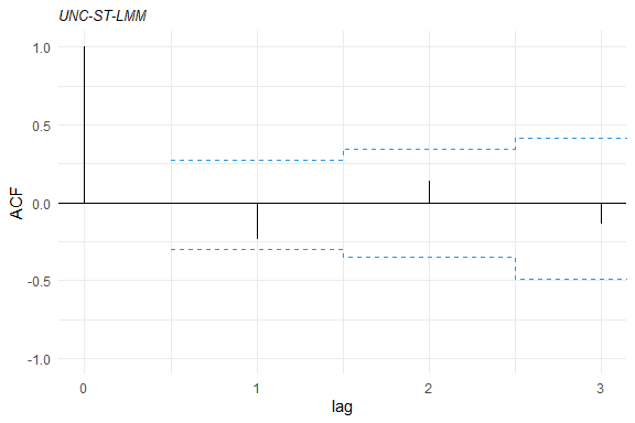
plot(mahalDist(fm1), nlabels = 2)
healy.plot(fm1, calcCI = TRUE)
#> Warning: `qplot()` was deprecated in ggplot2 3.4.0.
#> ℹ The deprecated feature was likely used in the skewlmm package.
#>   Please report the issue at
#>   <https://github.com/fernandalschumacher/skewlmm/issues>.
#> This warning is displayed once per session.
#> Call `lifecycle::last_lifecycle_warnings()` to see where this warning was
#> generated.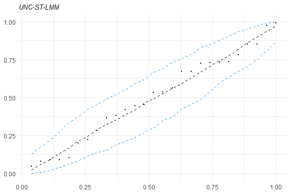
Furthermore, to fit a SMN-LMM one can use the following:
fm2 <- smn.lmm(dat1, formFixed = distance ~ age, formRandom = ~ age,
               groupVar = "Subject", distr = "t",
               control = lmmControl(quiet = TRUE))
summary(fm2)
#> Linear mixed models with distribution t and dependence structure UNC
#> Call:
#> smn.lmm(data = dat1, formFixed = distance ~ age, groupVar = "Subject",
#>     formRandom = ~age, distr = "t", control = lmmControl(quiet = TRUE))
#>
#> Distribution t with nu = 4.966122
#>
#> Random effects:
#>   Formula: ~age
#>   Structure:
#>   Estimated variance (D):
#>             (Intercept)         age
#> (Intercept)   3.2735098 -0.16423589
#> age          -0.1642359  0.03246643
#>
#> Fixed effects: distance ~ age
#> with approximate confidence intervals
#>                 Value  Std.error CI 95% lower CI 95% upper
#> (Intercept) 17.274030 0.67741340   15.9463240   18.6017357
#> age          0.593514 0.06218718    0.4716294    0.7153986
#>
#> Dependence structure: UNC
#>   Estimate(s):
#>    sigma2
#> 0.8926729
#>
#> Model selection criteria:
#>    logLik     AIC     BIC
#>  -211.351 436.701 455.476
#>
#> Number of observations: 108
#> Number of groups: 27
Now, for performing a LRT for testing if the skewness parameter is 0 (\(\text{H}_0: \lambda_i=0, \forall i\)), one can use the following:
lr.test(fm1,fm2)
#>
#> Model selection criteria:
#>       logLik     AIC     BIC
#> fm1 -209.837 437.675 461.814
#> fm2 -211.351 436.701 455.476
#>
#>     Likelihood-ratio Test
#>
#> chi-square statistics =  3.026434
#> df =  2
#> p-value =  0.2202005
#>
#> The null hypothesis that both models represent the
#> data equally well is not rejected at level  0.05
By default, the functions smsn.lmm and
smn.lmm now use the DAAREM method (a method for EM
acceleration, for details see help(package="daarem")) for
estimation, to improve the computational performance. This method
usually greatly reduces the convergence time, but its use can result in
numerical errors, specially for small samples. In this cases, the EM
algorithm can be used, as follows:
fm2EM <- smn.lmm(dat1, formFixed = distance ~ age, formRandom = ~ age, distr = 't',
                 groupVar = "Subject", control = lmmControl(algorithm = "EM",
                                                            quiet = TRUE))
fm2EM
#> Linear mixed models with distribution t and dependence structure UNC
#> Log-likelihood value at convergence: -211.3506
#> Distribution t with nu = 4.988346
#>
#> Fixed: distance ~ age
#> (Intercept)         age
#>  17.2875938   0.5958205
#> Random effects:
#>   Formula: ~ age by Subject
#>   Structure: General positive-definite
#>   Estimated variance (D):
#>             (Intercept)        age
#> (Intercept)   3.1584628 -0.1533659
#> age          -0.1533659  0.0314773
#> Error dependence structure: UNC
#>   Estimate(s):
#>    sigma2
#> 0.8982378
#> Number of observations: 108
#> Number of groups: 27
Also, we can fit a t-LMM with diagonal scale matrix for the random effects by using:
fm2diag <- update(fm2, covRandom = "pdDiag")
fm2diag
#> Linear mixed models with distribution t and dependence structure UNC
#> Log-likelihood value at convergence: -211.5985
#> Distribution t with nu = 4.984128
#>
#> Fixed: distance ~ age
#> (Intercept)         age
#>   17.282721    0.595894
#> Random effects:
#>   Formula: ~ age by Subject
#>   Structure: Diagonal
#>   Estimated variance (D):
#>             (Intercept)        age
#> (Intercept)    1.546268 0.00000000
#> age            0.000000 0.01789115
#> Error dependence structure: UNC
#>   Estimate(s):
#>    sigma2
#> 0.9698679
#> Number of observations: 108
#> Number of groups: 27
We can compare the information criteria for all fitted models using
the criteria function, as follows:
criteria(list(`ST-LMM` = fm1, `t-LMM` = fm2, `t-LMM(EM)` = fm2EM, `t-LMM-diag` = fm2diag))
#>               logLik npar      AIC      BIC
#> ST-LMM     -209.8374    9 437.6748 461.8140
#> t-LMM      -211.3506    7 436.7012 455.4761
#> t-LMM(EM)  -211.3506    7 436.7013 455.4762
#> t-LMM-diag -211.5985    6 435.1969 451.2897
For more examples, see help(smsn.lmm) and
help(smn.lmm).
An extension of the methods to account for censoring in SMSN-LMM is
under development. Tools for accommodating left, right, or interval
censored observations in the symmetrical family SMN-LMM (function
smn.clmm) are temporarily unavailable on CRAN, since they
depend on a package that was archived. They will be restored in a future
release.
For more information on censored models, we refer to Matos, L. A., Prates, M. O., Chen, M. H., and Lachos, V. H. (2013). Likelihood-based inference for mixed-effects models with censored response using the multivariate-t distribution. Statistica Sinica. DOI: 10.5705/ss.2012.043.